Land Cover Classification & Change Detection from Satellites

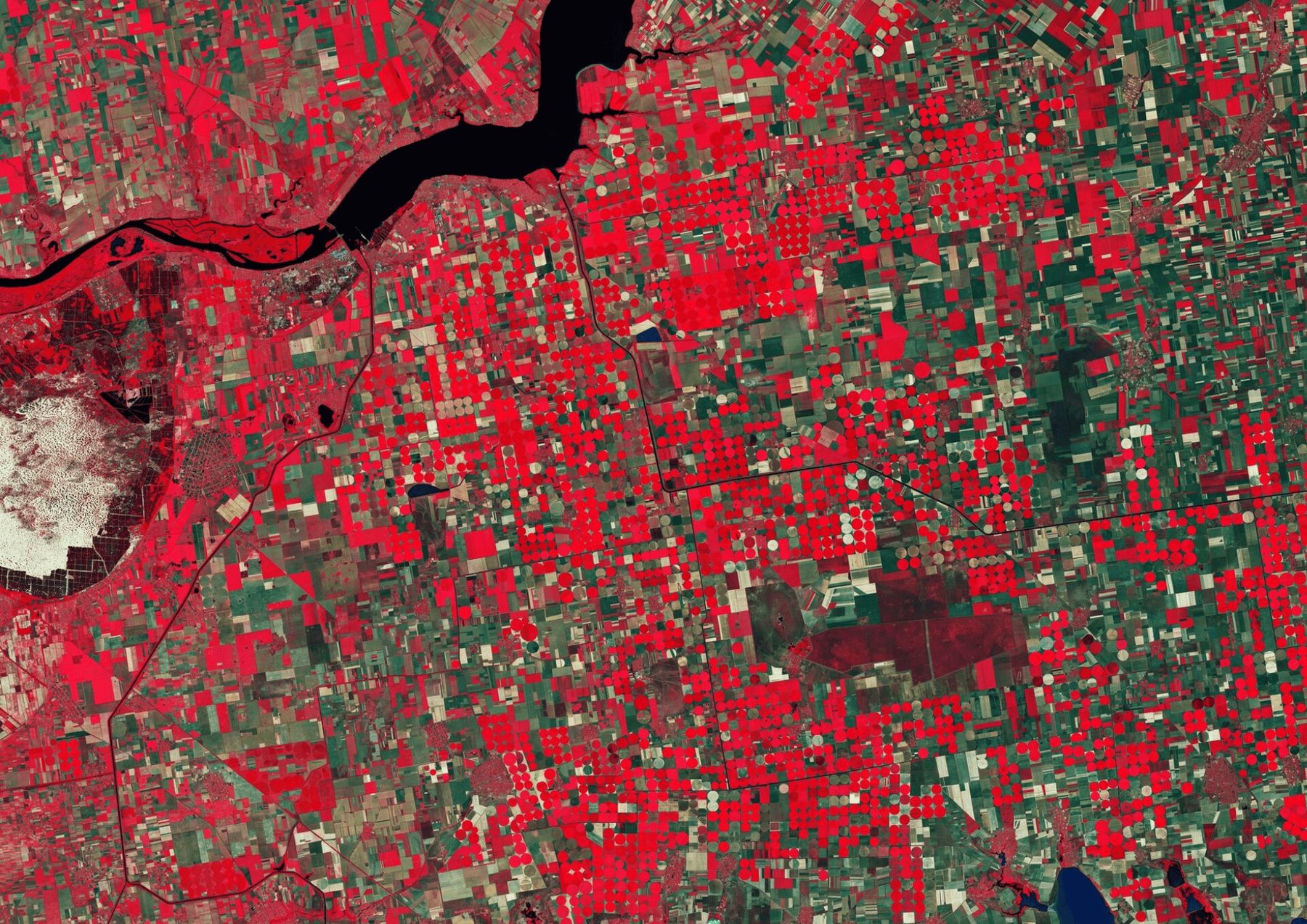
A satellite image is not a map. It is a grid of reflectance values that only becomes useful when you turn it into thematic classes — forest, cropland, built-up, water, bare soil — and when you can say, with defensible numbers, how those classes have changed over time. Land cover classification and change detection are the discipline that gets you there. They are the foundation beneath carbon accounting, agricultural monitoring, urban planning and environmental compliance, and they are far more demanding than pressing a "classify" button.

This post walks through the full pipeline the way we run it on real projects: the preprocessing everyone underestimates, the classification families and when each one earns its place, why accuracy assessment is a deliverable rather than an afterthought, and the change-detection algorithms that separate signal from noise across decades of imagery.

Preprocessing: the work that decides everything downstream

Most classification failures are not model failures. They are preprocessing failures. Before a single pixel is labelled, imagery has to be made physically comparable across scenes, dates and sensors. That means:

• Atmospheric correction — converting top-of-atmosphere radiance to surface reflectance so that a forest looks like a forest whether it was imaged in January or July.
• Cloud and shadow masking — clouds and their shadows are the single largest source of spurious "change." Robust masks, and cloud-free compositing over a time window, are non-negotiable.
• Mosaicking and co-registration — stitching adjacent scenes and aligning them precisely so pixels from different dates actually describe the same ground.
• Spectral indices — derived bands that amplify the signal you care about. NDVI for vegetation vigour, NDWI for water and moisture, NDBI for built-up surfaces. These indices frequently do more classification work than any clever model.

Get this stage right and a simple classifier performs well. Get it wrong and no algorithm will save you.

The classification families

There is no single best method — there is a best method for your resolution, your classes and your available training data. The main families:

• Unsupervised clustering groups pixels by spectral similarity with no training labels, then you assign meaning to the clusters. Fast for reconnaissance and for landscapes you don't yet understand.
• Supervised classifiers learn from labelled samples. Random forest, gradient boosting and support vector machines, run over stacked spectral bands, indices and temporal features, are the reliable workhorses for medium-resolution mapping. Temporal features — how a pixel's greenness moves through the seasons — are often what separates crops from grassland or evergreen from deciduous forest.
• Object-based image analysis (OBIA) segments high-resolution imagery into meaningful objects — a building, a field, a tree crown — and classifies those objects rather than individual pixels. Essential for sub-metre and aerial data, where per-pixel methods produce salt-and-pepper noise.
• Deep learning is the modern frontier, especially convolutional and transformer architectures that learn spatial context directly from the imagery. It shines on very high-resolution scenes and complex targets. We treat it as its own subject; if you want the detail, see our companion piece on machine learning on satellite imagery.

Accuracy assessment is the product

In carbon markets, compliance reporting and any setting where a map becomes evidence, the error bars are the deliverable. A map without a rigorous accuracy statement is an opinion. Proper assessment rests on a probability-based reference sample and a confusion matrix, from which you report:

• Overall accuracy — the share of reference points classified correctly.
• Producer's accuracy — how often real features of a class were captured (a measure of omission).
• User's accuracy — how often a mapped class is actually that class on the ground (a measure of commission).
• Area-adjusted estimates with confidence intervals — corrected area figures with explicit uncertainty, rather than naïve pixel counts that inherit every classification error.

This is exactly the discipline that underpins credible carbon work; it is the same rigour we brought to the Chaco Vivo REDD+ carbon project, where the defensibility of the change estimate was the entire point.

Change detection: finding real change, not noise

Once you can classify one date reliably, the harder question is how the landscape moves between dates. The main approaches, in increasing sophistication:

1. Post-classification comparison — classify each date independently and difference the maps. Intuitive and class-specific, but it compounds the error of both maps.
2. Spectral change detection — compare reflectance or indices directly to flag where something changed, before deciding what it changed into. Sensitive, but needs careful thresholds to avoid chasing phenology and illumination differences.
3. Time-series algorithms — the modern standard for long records. LandTrendr fits temporal trajectories and captures gradual trends and abrupt disturbances; CCDC (Continuous Change Detection and Classification) models each pixel's time series and detects breaks continuously; BFAST decomposes series into trend and seasonal components to locate breakpoints. These methods separate a real clearing event from seasonal green-up.

Those algorithms drive the applications buyers actually care about: deforestation and forest-degradation monitoring, urban expansion, crop and rangeland monitoring, disaster damage assessment, and surface-water change. And thanks to cloud platforms such as Google Earth Engine, continental-scale, multi-decade analysis that once required a server room now runs from a laptop.

From change map to decision

A classified map is rarely the end goal — it is an input. Land cover and its rate of change feed directly into suitability and siting models: where to expand, protect, restore or avoid. That is where classification connects to structured decision-making, and to our broader work on multi-criteria decision analysis in GIS, in which land cover is one weighted criterion among many.

Data sources

Open & public

• Sentinel-2 — 10 m optical, ~5-day revisit; the default workhorse for land cover.
• Landsat 8/9 — 30 m; the current sensors in a Landsat archive reaching back to 1972, which makes multi-decade change detection possible.
• Sentinel-1 SAR — radar that penetrates cloud, invaluable in the tropics and for all-weather monitoring.
• MODIS / VIIRS — daily but coarse; ideal for large-area, high-frequency trends.
• NAIP — high-resolution US aerial imagery.
• Ready-made products — ESA WorldCover, Dynamic World, Global Forest Change and the JRC Tropical Moist Forest (TMF) dataset, useful as baselines and cross-checks.

Commercial

• Planet — PlanetScope daily imagery at 3–5 m, plus higher-resolution SkySat tasking.
• Airbus — SPOT and Pléiades.
• Maxar — very high resolution down to 30–50 cm.
• Commercial SAR — Capella, ICEYE and Umbra.
• Impact Observatory — commercial land cover products.
• Nearmap / Vexcel — high-resolution aerial imagery.

Tools

• Google Earth Engine for planetary-scale processing.
• QGIS for desktop GIS and cartography.
• SNAP for Sentinel and SAR processing.
• Python (rasterio, scikit-learn) and R (terra) for custom pipelines and modelling.

Seeing the change

The most persuasive way to communicate all of this is not a static figure but an interactive before/after view: a swipe control that reveals two satellite dates over the same ground, paired with a derived change map that highlights exactly where cover was lost or gained. It turns a technical result into something a stakeholder can grasp in seconds and interrogate for themselves. Cartolytic builds these interactive change viewers as part of our delivery — the analysis is rigorous underneath, and the presentation makes the finding undeniable.

Whether the goal is a carbon baseline, an agricultural monitoring programme or an urban-growth study, the pattern is the same: disciplined preprocessing, a fit-for-purpose classifier, honest accuracy numbers, and time-series change detection that reports real change rather than noise. That is how imagery becomes decisions you can defend.