Machine Learning Models on Satellite Data for Detection

Detecting things from space — buildings, ships, solar panels, deforestation fronts, flood extent, illegal mining — used to mean an analyst painstakingly digitising features by hand. Machine learning changes the economics of that work entirely: it scales detection across continents and revisit cycles that no human team could ever cover manually. But the model is not the interesting decision. The interesting decision is the task, because the task dictates the architecture, the training data, and the standard of proof you need before anyone trusts the output.

Start with the task, not the model

Almost every operational request we get maps onto one of a handful of computer-vision task types. Choosing the right one is the first and most consequential design decision.

Scene classification

The simplest task: assign a single label to a whole image tile. Is this chip forest, urban, water, cropland? Scene classification is fast and cheap, and is often enough when you need coarse wall-to-wall coverage or a first-pass filter before running something heavier.

Semantic segmentation

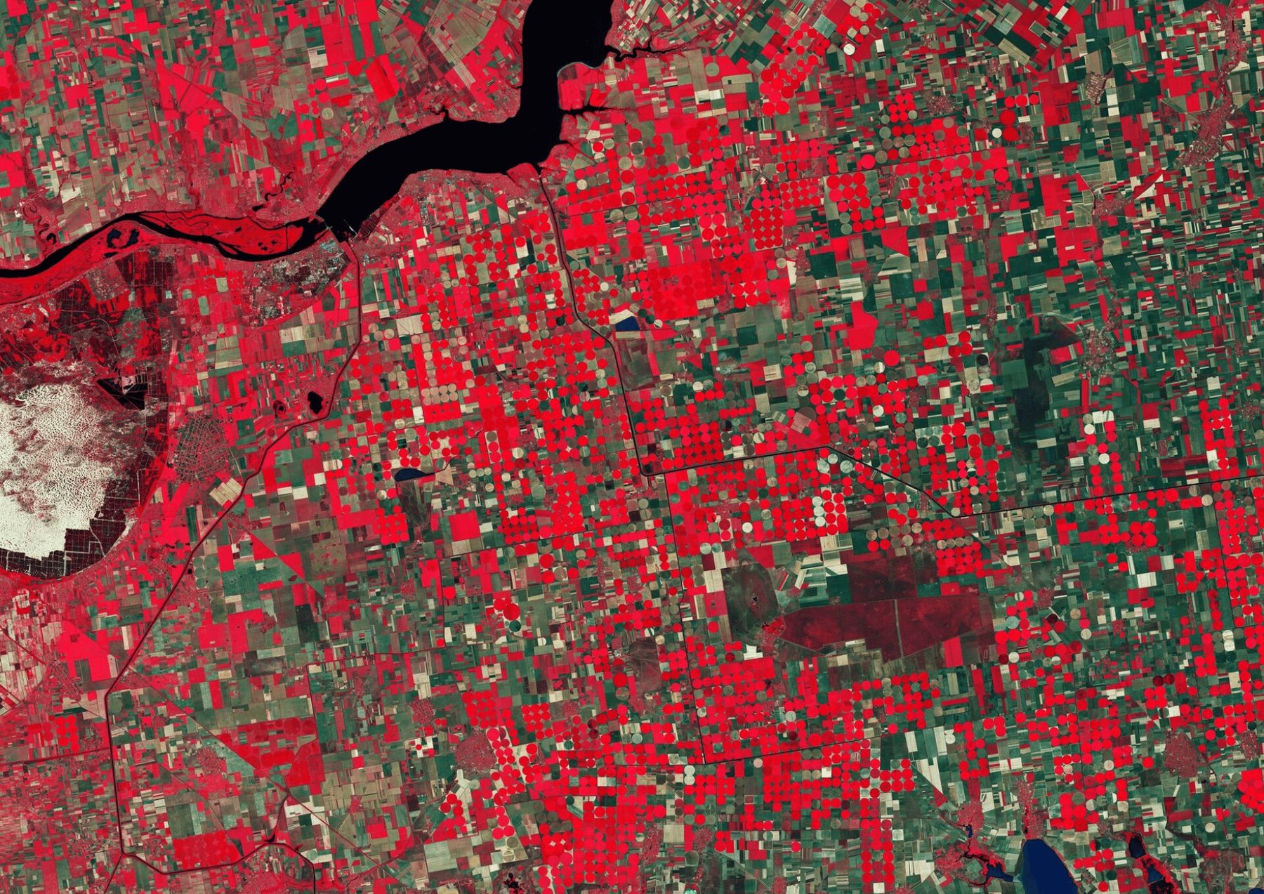
Segmentation labels every pixel, which is what you want for continuous phenomena: land cover, crop type, road networks, water, burn scars, flood extent. The workhorse architectures are encoder–decoder networks such as U-Net, DeepLabv3+ and SegFormer. This is the same family of models behind the modern approach to land-cover classification and change detection, where per-pixel output is the whole point.

Object detection and instance segmentation

When you need to find and delineate discrete things — individual buildings, vehicles, ships, aircraft, storage tanks, solar panels, informal settlements, illegal mining or logging — you move to object detection and instance segmentation. The YOLO family and Faster/Mask R-CNN dominate here. Overhead imagery has a specific twist: objects appear at arbitrary rotations, so oriented-bounding-box detectors that predict a rotation angle substantially outperform axis-aligned boxes on things like packed vehicles or ships at a quay.

Change and anomaly detection

Detecting what is different between two dates is its own task. Siamese networks compare co-registered image pairs and flag new construction, deforestation or disaster damage. Anomaly detection goes further, surfacing rare, novel events that no label set anticipated — useful precisely when you cannot enumerate in advance what you are looking for.

The foundation-model shift

The larger change reshaping the field is the arrival of geospatial foundation models: networks pretrained on enormous unlabelled Earth-observation archives, then fine-tuned for a specific task with only a handful of labels. The practical benefit is label efficiency, and that is decisive for niche detection problems where training labels barely exist.

The current working set worth naming includes:

• Prithvi and Prithvi-EO-2.0 (NASA and IBM) — a Vision Transformer trained on Harmonized Landsat–Sentinel imagery, with temporal and multi-band inputs.
• Clay — an open-source, multi-sensor model.
• SatMAE — a masked-autoencoder approach for satellite imagery.
• TerraMind (IBM and ESA) — jointly trained across optical, SAR and elevation data.
• AlphaEarth Foundations (Google DeepMind) — produces reusable embeddings for global mapping from sparse labels.
• Segment Anything Model (Meta), adapted for geospatial use — enables prompt-based feature extraction.

An honest caveat belongs here: no single model dominates. The right choice depends on the sensor, the spatial resolution and the task. A model that excels at optical land cover over Europe may be the wrong starting point for SAR flood mapping in the tropics. Treat the foundation model as a strong, label-efficient prior — not a guarantee.

An interactive detection overlay

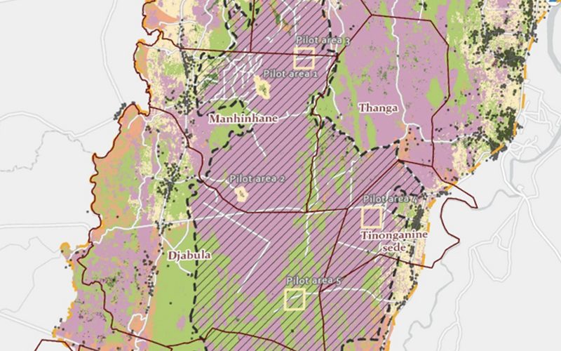
The clearest way to communicate what these models produce is to show it. A detection overlay — say, detected buildings or solar panels drawn over a real scene, or a before/after segmentation swipe — makes the output legible in a way that accuracy tables never do. The critical detail is that good model output is not a heatmap or a coloured raster; it is clean GIS vectors: closed polygons with attributes, ready to query, measure and join to other data. At Cartolytic we build exactly these kinds of interactive, clearly-labelled demonstrations so stakeholders can see detections as the analysable map layers they will actually work with, rather than as a black-box image. This is the same argument we make for interactive web maps over static reports.

A workflow that stands up to scrutiny

Scaling detection is only valuable if the results are trustworthy, and trust comes from the workflow, not the model card. The sequence we hold to:

1. Define the target precisely. What counts as a positive? Edge cases decide your labelling scheme and your metrics.
2. Source imagery at adequate resolution and revisit. You cannot detect a car in 10 m Sentinel-2 pixels; you cannot monitor daily change with an annual mosaic. Sensor choice is a hard constraint, not a preference.
3. Label — or borrow embeddings. Either annotate a training set or fine-tune a pretrained foundation model, leaning on its embeddings to cut labelling cost.
4. Fine-tune for the specific task and geography.
5. Validate carefully with the right metrics — precision, recall, mAP for detection, IoU for segmentation — on a spatially held-out test set.
6. Deploy at scale with tiled GPU inference, then post-process predictions into clean vector GIS layers.

The validation step carries the most weight and is the one most often done wrong. Spatial autocorrelation means nearby pixels are not independent, so a naïve random train/test split leaks information across the boundary and flatters the model with optimistic scores. A spatially blocked split — holding out entire regions — is the only honest way to estimate how the model generalises to ground it has never seen.

Data sources

Open & public

• Imagery: Sentinel-2, Sentinel-1 SAR, Landsat, HLS (Harmonized Landsat–Sentinel), NAIP.
• Labelled training sets: SpaceNet (buildings/roads), xView and xView2 (objects/damage), DOTA (oriented objects), BigEarthNet, EuroSAT, fMoW, Sen1Floods11, EuroCrops.
• Catalogues: Radiant MLHub / Source Cooperative, Hugging Face, Microsoft Planetary Computer, Google Earth Engine.

Commercial

• Higher-resolution / higher-revisit imagery for object detection: Planet, Maxar, Airbus, Satellogic.
• Commercial SAR: Capella, ICEYE, Umbra.
• Labelling services: Kili, Scale, Labelbox.

Tools

• TorchGeo, Raster Vision, TerraTorch (for Prithvi fine-tuning), segment-geospatial (SamGeo), eo-learn.
• PyTorch and TensorFlow.
• QGIS Deepness plugin, Google Earth Engine.

Where this fits

Machine learning scales detection dramatically, but it augments domain expertise and QA rather than replacing them. The continuous, automated monitoring behind credible carbon MRV (measurement, reporting and verification) — the kind underpinning our work on accurate carbon credits at Chaco Vivo — leans directly on this pipeline, but only because every detection is held to the same standard of proof that makes a compliance map defensible. And the vector layers these models produce rarely stand alone; they become inputs to the weighted trade-offs of multi-criteria decision analysis, where detection becomes evidence and evidence becomes a decision. The model is powerful. The rigour is what makes it usable.